Power Network System tutorial
Overview
In this tutorial you will:
|
Requirements
The example is available in the Examples/PNS folder of the toolbox.
Run
showdemo PNS_start
to open it, or
echodemo PNS_start
for an interactive demo.
Step 1
Power Network System Model
- Download problem data (download link), and extract the four .mat files in the current Matlab directory.
- Load state-space A, B, C, D matrices for the 4 Areas:
load('PNS_SS_matrices');
- Create a cell array of state-space discrete systems with sampling time 1s:
for i = 1:4
sys{i} = c2d(ss(A{i},B{i},C{i},D{i}),1);
end
- Add signal names (IMPORTANT. LSmodel class uses signal names to find interconnections and set signal limits):
load('PNS_signal_names');
for i = 1:4
sys{i}.InputName = name_inputs{i};
sys{i}.StateName = name_states{i};
sys{i}.OutputName = name_states{i};
end
- Build the LSmodel from the SS representation, specifying external inputs and outputs (internal connections are automatically generated by matching signal names):
model = LSmodel(sys, 0, name_external_inputs, name_external_outputs)
- Add signal limits with the set_sig_lim method, passing signal name, lower bound, and upper bound as arguments:
load('PNS_signal_limits');
for i = 1:length(name_external_inputs)/2
model = model.set_sig_lim(name_external_inputs((i-1)*2+1),-DrefMIN(i),DrefMAX(i));
end
for i = 1:length(name_external_outputs)/4
model = model.set_sig_lim(name_external_outputs((i-1)*4+1),-DtetaMIN(i),DtetaMAX(i));
end
Step 2
H2T object and control parameters
- Build H2T object passing the model as argument to the constructor:
h2t_obj = h2t(model)
- Check parameters required by the PnPMPC toolbox:
h2t_obj.checkParameters('PnPMPC')
You will see that the following parameters are missing:
- required: prediction horizon, k, input and output types;
- facultative: YALMIP settings.
- For an explanation about their meaning, check the following PnPMPC help page:
help createCtrlPnPMPC4lsmodel
- Load parameters from problem data:
load('PNS_control_parameters')
- Set generic parameters:
h2t_obj.setParameters('PredictionHorizon', N, 'StateWeights', Q, 'InputWeights', R)
Note how weights can be passed as scalar. In this case the weight will be automatically multiplied by an identity matrix of proper dimensions.
- Set PnPMPC-related parameters:
h2t_obj.setParameters('k', k, 'm', m, 'p', p, 'sdpsettings', sdp)
- Check parameters required by the MPT toolbox:
h2t_obj.checkParameters('MPT')
You will see that no additional parameters are required to build the MPT controller.
Step 3
PnPMPC decentralized controllers
- Build PnPMPC controllers (if you get a Java Exception here, just run command again):
ctrl_pnpmpc = h2t_obj.buildController('PnPMPC')
You will get an array of four controller objects, one for each Area of the Power Network System.
- Set zero-terminal constraint:
for i = 1:4
ctrl_pnpmpc(i) = ctrl_pnpmpc(i).zeroTerminal(Q((1:4),(1:4)), R)
end
- Controllers are now ready, and can be used to compute the control action for a given system state:
x = .05*rand(4,1)
u = ctrl_pnpmpc(1).uRH( x )
Step 4
MPT soft and aggressive controllers
- Set weights for soft controller:
h2t_obj.setParameters('StateWeights', 1, 'InputWeights', 1)
- Build soft MPT controller:
ctrl_mpt_soft = h2t_obj.buildController('MPT')
MPT object comes with the simulate method to easily perform closed-loop simulations.
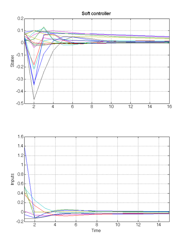
- Perform a 15-seconds closed-loop simulation starting from a random initial condition:
x0 = 0.1*rand(16,1);
closedloop_data_soft = ctrl_mpt_soft.simulate(x0, 15)
Plot state and input trajectories:
figure(1), subplot(211)
plot(closedloop_data_soft.X')
title('Soft controller'), ylabel('States')
subplot(212)
plot(closedloop_data_soft.U')
ylabel('Inputs'), xlabel('Time')
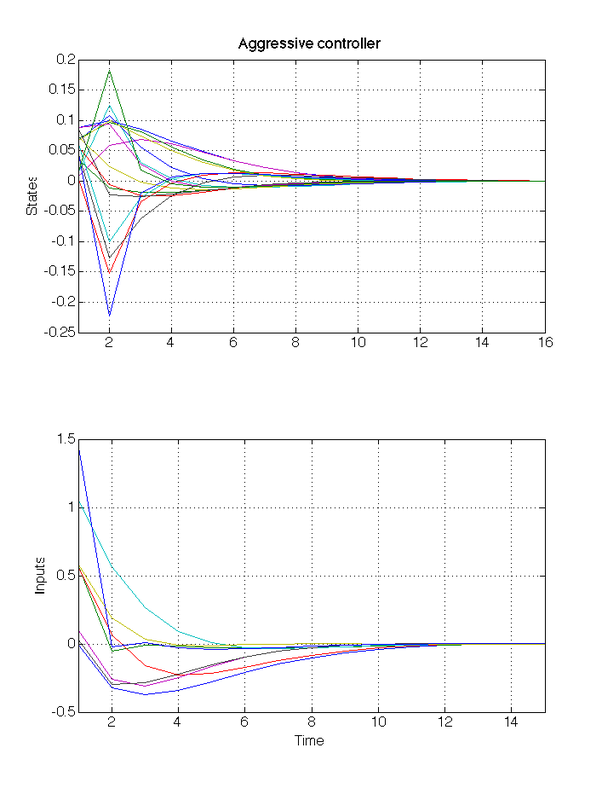
- Change parameters and build a more aggressive controller:
h2t_obj.setParameters('StateWeights', 10, 'InputWeights', 0.1)
ctrl_mpt_aggressive = h2t_obj.buildController('MPT')
- Perform a new closed-loop simulation and plot the results:
closedloop_data_aggressive = ctrl_mpt_aggressive.simulate(x0, 15)
figure(2), subplot(211)
plot(closedloop_data_aggressive.X')
title('Aggressive controller'), ylabel('States')
subplot(212)
plot(closedloop_data_aggressive.U')
ylabel('Inputs'), xlabel('Time')
At the end, you should get something similar to the following figures.
|
|