Masses tutorial
Overview
In this tutorial you will:
|
Requirements
The example is available in the Examples/Masses folder of the toolbox.
Run
showdemo Masses_start
to open it, or
echodemo Masses_start
for an interactive demo.
Step 1
System Model
- Set physical parameters, where 'M' is the number of masses, 'm' is the mass, 'k' and 'c the spring and damping coefficients, respectively:
M = 3; , m = 1; , k = 1.5; , c = 1;
- Set the number of states (position and velocity for each mass) and the number of inputs:
nx = 2*M; , nu = M-1;
- Build the continuous-time matrices:
Ac = full( [zeros(M,M) eye(M) gallery('tridiag',M,k/m,-2*k/m,k/m) gallery('tridiag',M,c/m,-c*k/m,c/m)] );
Bc = full( [zeros(M,M-1); gallery('tridiag',M-1,-1/m,1/m,0); zeros(1,M-2) -1/m] );
Cc = eye(nx);
- Create the standard SS system object discretizing with 0.5s sampling time:
sys = c2d( ss(Ac, Bc, Cc, 0), 0.5)
- Add signal names to the InputName, StateName and OutputName attributes of the standard SS object:
for i = 1:nu
sys.InputName(i) = { strcat('actuator', int2str(i)) };
end
for i = 1:M
sys.StateName(i) = { strcat('pos', int2str(i)) };
sys.OutputName(i) = { strcat('pos', int2str(i)) };
end
for i = (M+1):nx
sys.StateName(i) = { strcat('vel', int2str(i-M)) };
sys.OutputName(i) = { strcat('vel', int2str(i-M)) };
end
- Build the LSmodel object passing the external inputs and outputs names, which in this case coincide with the input and state names, respectively:
model = LSmodel(sys, sys.InputName, sys.StateName);
- Add signal limits with set_sig_lim method by matching signal names (for this example, we want to bound inputs between +1 and -1, and states between +4 and -4):
for i = 1:nu
model = model.set_sig_lim(strcat('actuator', int2str(i)), -1, 1);
end
for i = 1:M
model = model.set_sig_lim(strcat('pos', int2str(i)), -4, +4);
end
for i = M+1:nx
model = model.set_sig_lim(strcat('vel', int2str(i-M)), -4, +4);
end
Step 2
H2T object and control parameters
- Build H2T object passing the model as argument to the constructor:
h2t_obj = h2t(model)
- Set prediction horizon and weights:
h2t_obj.setParameters('PredictionHorizon', 10, 'StateWeights', 1, 'InputWeights', 0.1)
Note how weights can be passed as scalar. In this case the weight will be automatically multiplied by an identity matrix of proper dimensions.
Step 3
Open-loop simulation
To start from this step, download the H2T object (download link) and the State-Space representation (download link).
- Initialize simulation data:
Tsim = 50;
x = zeros(nx,Tsim); , x(:,1) = [3 -2 1 0 0 0]';
u = zeros(nu,Tsim);
- Open-loop evolution:
for i = 2:Tsim
x(:,i) = sys.A*x(:,i-1) + sys.B*u(:,i-1);
end
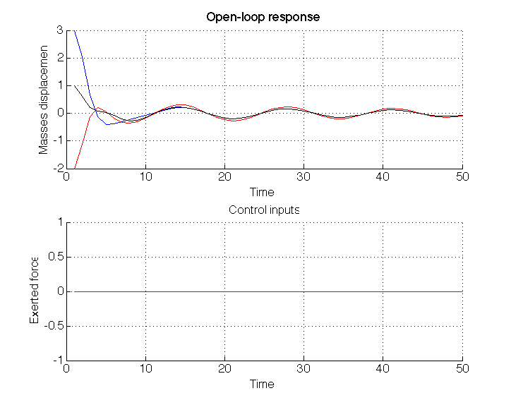
- Plot results:
figure(1), subplot(211)
hold on
plot(x(1,:)), plot(x(2,:),'r'), plot(x(3,:),'k')
title('Open-loop response'), xlabel('Time'), ylabel('Masses displacement')
subplot(212)
hold on
plot(u(1,:)), plot(u(2,:),'r')
title('Control inputs'), xlabel('Time'), ylabel('Exerted force')
You should get something similar to the following figure.
Step 4
MPT controller
To start from this step, download the H2T object (download link) and the State-Space representation (download link).
- Check parameters for MPT controller:
h2t_obj.checkParameters('MPT');
You should see that all parameters are ready.
- Build MPT controller:
ctrlMPT = h2t_obj.buildController('MPT');
- Initialize simulation data:
Tsim = 50;
x = zeros(nx,Tsim); , x(:,1) = [3 -2 1 0 0 0]';
u = zeros(nu,Tsim);
- Run closed loop simulation, computing the control input with the evaluate method of the MPT controller object:
for i = 2:Tsim
u(:,i-1) = ctrlMPT.evaluate(x(:,i-1));
x(:,i) = sys.A*x(:,i-1) + sys.B*u(:,i-1);
end
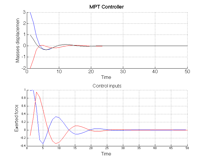
Plot state and input trajectories:
figure(2), subplot(211)
hold on
plot(x(1,:)), plot(x(2,:),'r'), plot(x(3,:),'k')
title('MPT Controller'), xlabel('Time'), ylabel('Masses displacement')
subplot(212)
hold on
plot(u(1,:)), plot(u(2,:),'r')
title('Control inputs'), xlabel('Time'), ylabel('Exerted force')
You should get something similar to the following figure.
Step 5
PnPMPC controller
To start from this step, download the H2T object (download link) and the State-Space representation (download link).
- Check parameters for PnPMPC controller:
h2t_obj.checkParameters('MPT');
- Set missing parameters (for an explanation of their meaning type 'help createCtrlPnPMPC4lsmodel'):
h2t_obj.setParameters('k', {10}, 'm', ones(nu,1) ,'p', ones(nx,1))
- Build PnPMPC controller and set zero-terminal constraint (if you get a Java Exception, simply run command again):
ctrlPnPMPC = h2t_obj.buildController('PnPMPC');
ctrlPnPMPC = ctrlPnPMPC.zeroTerminal(eye(nx), eye(nu));
- Initialize simulation data:
Tsim = 50;
x = zeros(nx,Tsim); , x(:,1) = [3 -2 1 0 0 0]';
u = zeros(nu,Tsim);
- Run closed loop simulation, computing the control input with the uRH method of the PnPMPC controller object:
for i = 2:Tsim
u(:,i-1) = ctrlPnPMPC.uRH(x(:,i-1));
x(:,i) = sys.A*x(:,i-1) + sys.B*u(:,i-1);
end
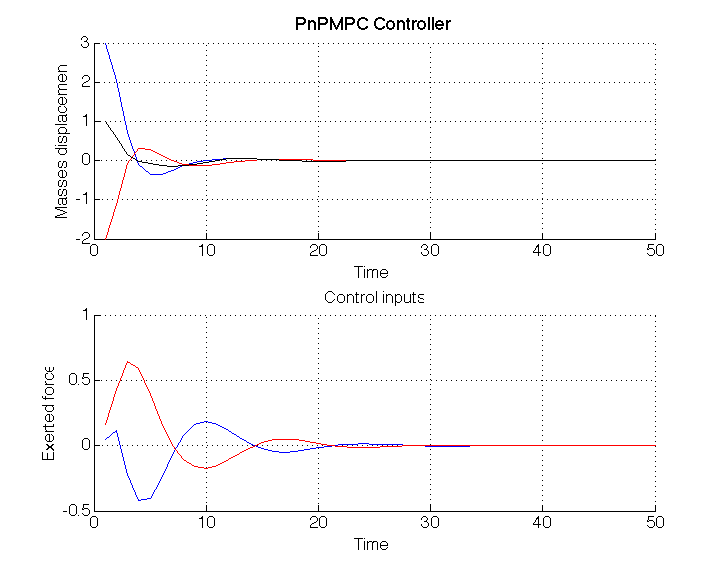
Plot state and input trajectories:
figure(3), subplot(211)
hold on
plot(x(1,:)), plot(x(2,:),'r'), plot(x(3,:),'k')
title('PnPMPC Controller'), xlabel('Time'), ylabel('Masses displacement')
subplot(212)
hold on
plot(u(1,:)), plot(u(2,:),'r')
title('Control inputs'), xlabel('Time'), ylabel('Exerted force')
You should get something similar to the following figure.